Tutorial

This tutorial is available as a Jupyter notebook that you can download at the link below so that you can follow along. In the web version, we show the output of the code as comments at the bottom, so that it can be copied and pasted without annoying extra characters. Additionally, every code block on the website (not just the tutorial) has a button at the top right corner to copy the entire content of the block.
This tutorial is focused on showing how to use the functionality available in CYTools. For more detailed background about the underlying objects, and the mathematical and physical motivations for these computations, we refer the reader to the CYTools paper (to appear).
In this tutorial, we will look at the basics of the CYTools package, as well as show a realistic use case. Let us start with a brief overview of the available classes.
Overview
The starting objects for most computations are the Polytope and Cone classes. These can be imported as follows.
(In case you are not familiar with Jupyter notebooks, the way you run the code in a cell is by first highlighting it and then pressing ctrl+enter.)
from cytools import Polytope, Cone
Other important classes in this package are Triangulation, ToricVariety, and CalabiYau. These should generally not be directly constructed by the user. Instead, objects of these classes can be constructed by designated functions from more fundamental objects.
Let us take a brief look at each of the classes and how to perform computations. After taking a look at each of the classes, we will give a self-contained example where we show how to perform computations.
Polytopes
First, let's take a look at the Polytope class. A Polytope object can be created by specifying a list of points defining the convex hull. Note that CYTools only supports lattice polytopes so any floating point numbers will be truncated to integers.
p = Polytope([[1,0,0,0],[0,1,0,0],[0,0,1,0],[0,0,0,1],[-1,-1,-1,-1]])
We can print some information about the polytope as follows.
print(p)
# A 4-dimensional reflexive lattice polytope in ZZ^4
The list of lattice points, boundary points, interior points, etc., can be computed using self-explanatory functions. For example, if we want the full list of points of the polytope, we can obtain it as follows.
p.points()
# array([[ 0,  0,  0,  0],
#        [-1, -1, -1, -1],
#        [ 0,  0,  0,  1],
#        [ 0,  0,  1,  0],
#        [ 0,  1,  0,  0],
#        [ 1,  0,  0,  0]])
As another example, if we want to find the 2-dimensional faces of the polytope, we can do so as follows.
p.faces(d=2)
# (A 2-dimensional face of a 4-dimensional polytope in ZZ^4,
#  A 2-dimensional face of a 4-dimensional polytope in ZZ^4,
#  A 2-dimensional face of a 4-dimensional polytope in ZZ^4,
#  A 2-dimensional face of a 4-dimensional polytope in ZZ^4,
#  A 2-dimensional face of a 4-dimensional polytope in ZZ^4,
#  A 2-dimensional face of a 4-dimensional polytope in ZZ^4,
#  A 2-dimensional face of a 4-dimensional polytope in ZZ^4,
#  A 2-dimensional face of a 4-dimensional polytope in ZZ^4,
#  A 2-dimensional face of a 4-dimensional polytope in ZZ^4,
#  A 2-dimensional face of a 4-dimensional polytope in ZZ^4)
Conveniently, the ordering of the faces dual polytopes is preserved by the duality. In other words, the dual of the th face of dimension of polytope is the th face of dimension of the dual polytope. We can verify this as follows.
n = 0 # Try changing the value of n
p.faces(d=2)[n].dual_face() is p.dual_polytope().faces(d=1)[n]
# True
We can compute information relevant to Batyrev's construction of Calabi-Yau hypersurfaces when the polytope is reflexive and 4-dimensional. To avoid ambiguity, one must specify if the polytope should be viewed as living in the lattice or the lattice.
p.h11(lattice="N"), p.h21(lattice="N")
# (1, 101)
To see the full list of available functions you can type the name of the polytope (in this case p) followed by a period and then press tab. This works for any kind of object! So if you want to see the available functions for ToricVariety, CalabiYau, or Cone objects you can do the same thing.
You can find the full documentation of the Polytope class here.
Using the Kreuzer-Skarke database
CYTools provides two useful functions to work with the Kreuzer-Skarke (KS) database. We can import them as follows.
from cytools import read_polytopes, fetch_polytopes
The first function takes a file name as input and reads all polytopes specified in the format used in the KS database. The second file directly fetches the polytopes from the database. For example let's fetch 100 polytopes with =7.
g = fetch_polytopes(h21=7, lattice="N", limit=100)
print(g)
# <generator object polytope_generator at 0x7f306eacaeb0>
As you can see above, these functions return generator objects that give one polytope at a time. To get the polytopes we can do the following.
p1 = next(g)
p2 = next(g)
Or to get the full list of polytopes we can do this.
l = list(g)
print(len(l))
# 98
In this example, the generator had a limit of 100 polytopes. Since in the previous cell it had already generated two polytopes, then once we constructed the list it only generated the remaining 98.
If you are not familiar with Python, it is worth noting that generators raise an exception once they reach the end. For this reason, if you are using the next function in your code it is usually necessary to wrap this with try-except statements as in the following example.
g = fetch_polytopes(h21=2, lattice="N", limit=100)
for i in range(100):
    try:
      p = next(g)
      print(f"Fetched polytope {i}")
    except StopIteration:
      print(f"Iteration stopped at number {i}")
      break
Alternatively, one can conveniently use generators in for-loops in the following way.
g = fetch_polytopes(h21=1, lattice="N", limit=100)
for p in g:
    print(p)
# A 4-dimensional reflexive lattice polytope in ZZ^4
# A 4-dimensional reflexive lattice polytope in ZZ^4
# A 4-dimensional reflexive lattice polytope in ZZ^4
# A 4-dimensional reflexive lattice polytope in ZZ^4
# A 4-dimensional reflexive lattice polytope in ZZ^4
The fetch_polytopes function can take many different parameters, and can even fetch 5D polytopes from the Schöller-Skarke database. To see more information about a function, you can write the name of the function and end it with a question mark (?), as follows. (This only works on Jupyter notebooks.)
fetch_polytopes?
You can find the documentation of the fetch_polytopes function here.
Triangulations
Let us now look at how we can triangulate the polytopes. We start with the following polytope.
p = Polytope([[1,0,0,0],[0,1,0,0],[0,0,1,0],[-3,-1,-1,0],[1,1,1,2],[-1,-1,1,-1],[-1,1,-1,-1]])
We can obtain a triangulation simply by using the following line.
t = p.triangulate()
And we can print information about the triangulation as follows.
print(t)
# A fine, regular, star triangulation of a 4-dimensional point configuration with 10 points in ZZ^4
For four-dimensional reflexive polytopes it defaults to constructing a fine, star, regular triangulation (FRST). Notice that it specifically tells us how many points there are in the triangulated point configurations. In this case, it has 10 points. Let us see how many lattice points the polytope contains.
len(p.points())
# 11
This mismatch is due to the fact that, for 4D reflexive polytopes, the triangulate function ignored points interiors to facets, as they correspond to toric divisors that do not intersect the Calabi-Yau hypersurface. When it is necessary to include the full set of points one can do so as follows.
p.triangulate(include_points_interior_to_facets=True)
# A fine, regular, star triangulation of a 4-dimensional point configuration with 11 points in ZZ^4
Other options such as heights, whether to make it a star, the backend, etc., can be inputted as well. In the following line we input a height vector, tell it to turn it into a star triangulatio, and specify CGAL as the software that will perform the triangulation.
t = p.triangulate(heights=[0,3,7,1,9,1,1,1,3,2,2], make_star=True, backend="cgal")
Various properties of the triangulation can be accessed by self-explanatory functions. For example, we can find the list of simplices as follows.
t.simplices()
# array([[0, 1, 2, 3, 6],
#        [0, 1, 2, 3, 9],
#        [0, 1, 2, 4, 7],
# ** output truncated **
Some functionality requires additional software that is installed as a dependency. For example, finding triangulations that differ by a bistellar flip requires TOPCOM.
t.neighbor_triangulations()
# [A fine, non-star triangulation of a 4-dimensional point configuration with 10 points in ZZ^4,
#  A fine, star triangulation of a 4-dimensional point configuration with 10 points in ZZ^4,
#  A non-fine, star triangulation of a 4-dimensional point configuration with 10 points in ZZ^4,
#  A fine, star triangulation of a 4-dimensional point configuration with 10 points in ZZ^4,
#  A fine, non-star triangulation of a 4-dimensional point configuration with 10 points in ZZ^4,
#  A non-fine, star triangulation of a 4-dimensional point configuration with 10 points in ZZ^4]
If one wants to generate random triangulations, one for example can pick random heights around the Delaunay triangulation. This can be done with the random_triangulations_fast function.
triangs_gen = p.random_triangulations_fast(N=100)
Again, a generator is returned instead of a list of triangulations for performance reasons.
The above method to find triangulations is fast, but does not produce a fair sampling of triangulations. This can be done with the random_triangulations_fair function.
You can find the full documentation of the Triangulation class here.
Toric Varieties
We can interpret star triangulations as defining a toric fan, and construct the associated toric variety. We can do this as follows.
p = Polytope([[1,0,0,0],[0,1,0,0],[0,0,1,0],[-1,1,1,0],[0,-1,-1,0],
              [0,0,0,1],[1,-2,1,1],[-2,2,0,-1],[1,0,-1,-1]])
t = p.triangulate()
v = t.get_toric_variety()
Basic information can be printed as follows.
print(v)
# A simplicial compact 4-dimensional toric variety with 31 affine patches
Various properties of the toric variety can be accessed by self-explanatory functions. For example, its intersection numbers and Mori cone can be computed as follows.
intnums = v.intersection_numbers()
mori_cone = v.mori_cone()
You can find the full documentation of the ToricVariety class here.
Calabi-Yaus
Let's now get to the class of most interest. A CalabiYau object can be obtained from a triangulation or from a toric variety as follows.
p = Polytope([[1,0,0,0],[0,1,0,0],[0,0,1,0],[-1,1,1,0],[0,-1,-1,0],[0,0,0,1],
              [1,-2,1,1],[-2,2,0,-1],[1,0,-1,-1]])
t = p.triangulate()
v = t.get_toric_variety()
cy = v.get_cy()
cy = t.get_cy() # This is equivalent to the line above, but you can get it directly from the triangulation
Basic information can be printed as follows.
print(cy)
# A Calabi-Yau 3-fold hypersurface with h11=7 and h21=23 in a 4-dimensional toric variety
Various properties of the CY can be accessed by self-explanatory functions. For example, its intersection numbers and the inherited part of the Mori cone from toric geometry can be computed as follows.
intnums = cy.intersection_numbers()
mori_cone = cy.toric_mori_cone()
You can find the full documentation of the CalabiYau class here.
Cones
Lastly, let's briefly look at the Cone class. These can be constructed by specifying a set of rays or normals to hyperplanes.
c1 = Cone([[0,1],[1,1]])
c2 = Cone(hyperplanes=[[0,1],[1,1]])
Let us look at the (toric) Mori cone of the above Calabi-Yau.
mc = cy.toric_mori_cone()
We can print some information about it as follows.
print(mc)
# A 7-dimensional rational polyhedral cone in RR^12 generated by 36 rays
Note that by default the Mori cone is given in a basis-independent way, as an dimensional cone in an -dimensional lattice. We can tell CYTools to use a basis of curves with the in_basis=True parameter. For more information of how to set a basis of curves or divisors see set_curve_basis or set_divisor_basis.
The Kähler cone can be computed from the designated function, or by taking the dual of the Mori cone in a basis of curves.
kc = cy.toric_kahler_cone()
kc = cy.toric_mori_cone(in_basis=True).dual() # This line is equivalent to the previous, but it is less direct
CYTools uses a lazy duality where no computation is done and instead the definition of the cone is dualized. This can be seen by printing the information and noticing that the cone is defined in terms of hyperplane normals instead of generating rays.
print(kc)
# A rational polyhedral cone in RR^7 defined by 36 hyperplanes.
However, we can still find the generating rays if desired, although the difficulty increases exponentially with dimension.
kc.rays()
# array([[ 0,  2,  2,  0,  3,  1,  1],
#        [ 0,  3,  3,  0,  3,  1,  1],
#        [ 0,  2,  4,  1,  3,  1,  1],
# **output truncated**
After finding the rays, the definition of the cone is updated to show the number of generating rays.
print(kc)
# A 7-dimensional rational polyhedral cone in RR^7 generated by 18 rays
As with other classes, there are numerous functions available for the Cone class. For example we can take intersections, find lattice points, and various other things. For example, we can find the tip of thestretched Kähler cone as follows. (Recall that this is defined as the shortest vector that is at least a distance , here , from every wall of the cone.)
tip = kc.tip_of_stretched_cone(1)
print(f"Tip is at {tip}\nthe minimum distance to a wall is {min(kc.hyperplanes().dot(tip))}")
# Tip is at [ 2. 10. 12.  1. 14.  5.  5.]
# the minimum distance to a wall is 0.9999999999999869
You can find the full documentation of the Cone class here.
Illustrative Example
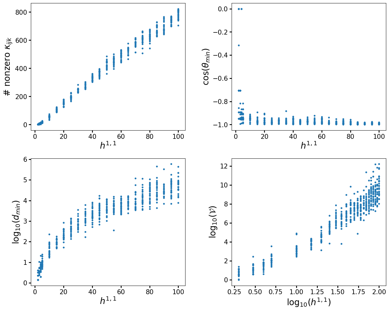
Let us now look at a full example computation. For this, let's reproduce some of the results of the paper The Kreuzer-Skarke Axiverse [1808.01282]. In particular, we will reproduce figures 1, 3, 4, and 8(a). We will be using a much smaller set of polytopes so that the code only takes a few minutes to run. Consequently, so the spread of the distributions will not be as large, but it is clear that they match. To more closely match the procedure used in the paper we will only construct a single triangulation per polytope using TOPCOM. However, we will also show how to sample triangulations for each polytope.
This code should take about 5 minutes to run.
# We start by importing fetch_polytopes,
# a plotting package, and numpy
from cytools import fetch_polytopes
import matplotlib.pyplot as plt
import numpy as np

# These are the settings for the scan.
# We scan h11=2,3,4,5,10,15,...,100
# For each h11 we take 25 polytopes
h11s = [2,3,4] + list(range(5,105,5))
n_polys = 25

# These are the lists where we will save the data
h11_list = []
nonzerointnums = []
costhetamin = []
dmins = []
Xvols = []

for h11 in h11s:
    print(f"Processing h11={h11}", end="\r")
    for p in fetch_polytopes(h11=h11, lattice="N",
                             favorable=True, limit=n_polys):
        # Here we use a single triangulation constructed using topcom,
        # to more closely reproduce the data in the paper.
        t = p.triangulate(backend="topcom")
        cy = t.get_cy()
        h11_list.append(h11)
        nonzerointnums.append(len(cy.intersection_numbers(in_basis=True)))
        mori_rays = cy.toric_mori_cone(in_basis=True).rays()
        mori_rays_norms = np.linalg.norm(mori_rays, axis=1)
        n_mori_rays = len(mori_rays)
        costhetamin.append(min(
            mori_rays[i].dot(mori_rays[j])
                /(mori_rays_norms[i]*mori_rays_norms[j])
            for i in range(n_mori_rays) for j in range(i+1,n_mori_rays)))
        tip = cy.toric_kahler_cone().tip_of_stretched_cone(1)
        dmins.append(np.log10(np.linalg.norm(tip)))
        Xvols.append(np.log10(cy.compute_cy_volume(tip)))
print("Finished processing all h11s!")
print(f"Scanned through {len(h11_list)} CY hypersurfaces.")

# We plot the data using matplotlib.
# If you are not familiar with this package, you can find tutorials and
# documentation at https://matplotlib.org/

xdata = [h11_list]*3 + [np.log10(h11_list)]
ydata = [nonzerointnums, costhetamin, dmins, Xvols]
xlabels = [r"$h^{1,1}$"]*3 + [r"log${}_{10}(h^{1,1})$"]
ylabels = [r"# nonzero $\kappa_{ijk}$", r"$\cos(\theta_{min})$",
           r"log${}_{10}(d_{min})$", r"log${}_{10}(\mathcal{V})$"]
fig, ax0 = plt.subplots(2, 2, figsize=(15,12))

for i,d in enumerate(ydata):
    ax = plt.subplot(221+i)
    ax.scatter(xdata[i], ydata[i], s=10)
    plt.xlabel(xlabels[i], size=20)
    plt.ylabel(ylabels[i], size=20)
    plt.tick_params(labelsize=15, width=2, length=5)

plt.subplots_adjust(wspace=0.3, hspace=0.22)
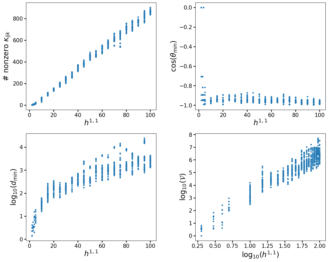
As we previously mentioned, in this example we restricted to finding only a single triangulation per polytope with TOPCOM, as this is how the original analysis was done. However, with CYTools we can do better, as there are functions to sample triangulations from polytopes. Let us redo the above computation, but now picking a small set of triangulations obtained by randomly picking heights, which is done by the random_triangulations_fast function. However, keep in mind that this does not produce a fair sampling of triangulations. For a fair sampling, one should using the much slower random_triangulations_fair function. However, for demonstration purposes, as well as for other applications like machine learning, a fast sampling of triangulations is sufficient.
Again, this code should only take about 5 minutes to run.
# We start by importing fetch_polytopes,
# a plotting package, and numpy
from cytools import fetch_polytopes
import matplotlib.pyplot as plt
import numpy as np

# These are the settings for the scan.
# We scan h11=2,3,4,5,10,15,...,100
# For each h111 we take 10 polytopes,
# and 5 random triangulations for each polytope
h11s = [2,3,4] + list(range(5,105,5))
n_polys = 10
n_triangs = 5

# These are the lists where we will save the data
h11_list = []
nonzerointnums = []
costhetamin = []
dmins = []
Xvols = []

for h11 in h11s:
    print(f"Processing h11={h11}", end="\r")
    for p in fetch_polytopes(h11=h11, lattice="N",
                             favorable=True, limit=n_polys):
        # Here we take a random set of triangulations by picking random heights.
        # We use the random_triangulations_fast function with max_retries=5 so
        # that the generation doesn't take too long. However, this will not
        # generate a fair sampling of the triangulations of the polytope.
        # For a fair sampling one should use the random_triangulations_fair
        # function, which is much slower.
        for t in p.random_triangulations_fast(N=n_triangs, max_retries=5):
            cy = t.get_cy()
            h11_list.append(h11)
            nonzerointnums.append(len(cy.intersection_numbers(in_basis=True)))
            mori_rays = cy.toric_mori_cone(in_basis=True).rays()
            mori_rays_norms = np.linalg.norm(mori_rays, axis=1)
            n_mori_rays = len(mori_rays)
            costhetamin.append(min(
                mori_rays[i].dot(mori_rays[j])
                    /(mori_rays_norms[i]*mori_rays_norms[j])
                for i in range(n_mori_rays) for j in range(i+1,n_mori_rays)))
            tip = cy.toric_kahler_cone().tip_of_stretched_cone(1)
            dmins.append(np.log10(np.linalg.norm(tip)))
            Xvols.append(np.log10(cy.compute_cy_volume(tip)))
print("Finished processing all h11s!")
print(f"Scanned through {len(h11_list)} CY hypersurfaces.")

# We plot the data using matplotlib.
# If you are not familiar with this package, you can find tutorials and
# documentation at https://matplotlib.org/

xdata = [h11_list]*3 + [np.log10(h11_list)]
ydata = [nonzerointnums, costhetamin, dmins, Xvols]
xlabels = [r"$h^{1,1}$"]*3 + [r"log${}_{10}(h^{1,1})$"]
ylabels = [r"# nonzero $\kappa_{ijk}$", r"$\cos(\theta_{min})$",
           r"log${}_{10}(d_{min})$", r"log${}_{10}(\mathcal{V})$"]
fig, ax0 = plt.subplots(2, 2, figsize=(15,12))

for i,d in enumerate(ydata):
    ax = plt.subplot(221+i)
    ax.scatter(xdata[i], ydata[i], s=10)
    plt.xlabel(xlabels[i], size=20)
    plt.ylabel(ylabels[i], size=20)
    plt.tick_params(labelsize=15, width=2, length=5)

plt.subplots_adjust(wspace=0.3, hspace=0.22)
The above example shows the power of CYTools. The original paper required very significant effort to assemble the code for the analysis, as it required downloading the KS database, performing some computations on SageMath, then performing some extra computations in Mathematica, and finally using a variety of scripts to gather together all the data. Now, anyone can perform the full analysis with a few lines of code in CYTools. Although we only took a small number of polytopes in this example, one could easily increase the range of the scan and even surpass the statistics of the original paper by running the computation on a standard laptop overnight.
This concludes the brief tutorial. We have some additional advanced usage instructions for people who intend to perform large-scale computations with CYTools. For a full list of available classes and functions please explore the documentation.